Analyzing the eigenvalues of a covariance matrix to identify multicollinearity

In this article, I’m reviewing a method to identify collinearity in data, in order to solve a regression problem. It’s important to note, there is more than one way to detect multicollinearity, such as the variance inflation factor, manually inspecting the correlation matrix, etc.

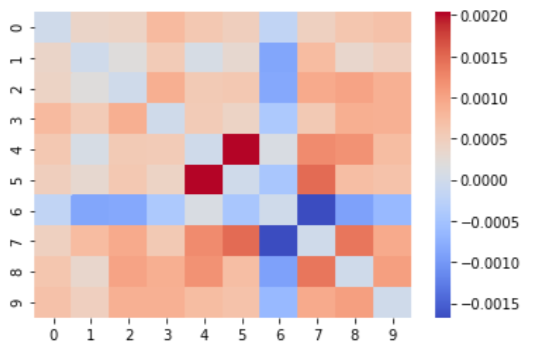
If we try to inspect the correlation matrix for a large set of predictors, this breaks down somewhat.

For example, using scikitlearn’s diabetes dataset:

Slightly interesting, but not very informative

Some of these data look correlated, but it’s hard to tell. I wouldn’t use this as our only method of identifying issues.

Multicollinearity can cause issues in understanding which of your predictors are significant as well as errors in using your model to predict out of sample data when the data do not share the same multicollinearity.

We need to begin by actually understanding each of these, in detail.

Multicollinearity

Let’s break it down.

We’ve taken a geometric term, and repurposed it as a machine learning term. The definition of colinear is:

However, in our use, we’re talking about correlated independent variables in a regression problem. That is, two variables are colinear, if there is a linear relationship between them.

E.g.

If X_2 = λ*X_1, then we say that X_1 and X_2 are colinear.

If you’re using derived features in your regressions, it’s likely that you’ve introduced collinearity. E.g adding another predictor X_3 = X1**2.

Occasionally, collinearity exists in naturally in the data.

Covariance

The covariance of two variables, is defined as the mean value of the product of their deviations. If the covariance is positive, then the variables tend to move together (if x increases, y increases), if negative, then they also move together, inversely (if x decreases, y increases), if 0, there is no relationship.

We want to distinguish this from correlation, which is just a standardized version of covariance that allows us to determine the strength of the relationship by bounding to -1 and 1. Covariance, on the other hand, is unbounded and gives us no information on the strength of the relationship.

Thanks to numpy, calculating a covariance matrix from a set of independent variables is easy!

First let’s look at the covariance matrix

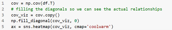
We can see that X_4 and X_5 have a relationship, as well as X_6 and X_7

The Eigenvalues of the Covariance Matrix

The eigenvalues and eigenvectors of this matrix give us new random vectors which capture the variance in the data.

If one/or more of the eigenvalues is close to zero, we’ve identified collinearity in the data.

Let’s take a look at this dataset:

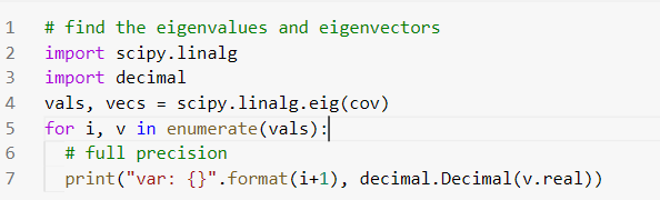
var: 1 0.00912520221242393847482787805347470566630363
var: 2 0.00338394157645012256391270355493361421395093202
var: 3 0.002734608416162503680829631846904703706968575 
var: 4 0.0021666131242379705647282950309318039217032492160 
var: 5 0.000019411632428624847835013991770303221073845634236931
var: 6 0.000177596168211303229037337225726389533519977703690
var: 7 0.00150155460147426297011497009492586585110984742641
var: 8 0.00098340862260182823444132349521851210738532245159
var: 9 0.0013667102288161217960721360853426631365437060594 
var: 10 0.001216690378645803819607218443366036808583885431

We see the most of the eigenvalues have small values, however, two of our eigenvalues have a very small value, which corresponds to the correlation of the variables we identified above.

Summary

Typically, in a small regression problem, we wouldn’t have to worry too much about collinearity. However, in cases where we are dealing with thousands of independent variables, this analysis becomes useful.

Hope you enjoyed!

If you found this article interesting, check out this:

Demystified: Kullback–Leibler Divergence